Depending on the data source, actuals and plan values might initially be loaded into two separate tables. The main reason for this is that, in many cases, plan values are prepared on a less granular level than actuals.
You might prepare the budget per month and organizational level (i.e. Business Units or similar) but in the Actuals, you also have daily data per Client, product, salesperson, etc. In order to set up a proper data model (learn more about the star schema), it’s best to combine Actuals and Plan data into one table.
As always, there are different ways to do this. In this article, we will focus on two different ways. One way is to physically combine the tables into one and the second is to combine the tables using the DAX function TREATAS.
Case 1: Combine tables in Power Query
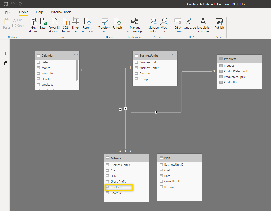
As you can see in the data model below, there are three lookup tables on top and two fact tables on the bottom. You can also see that in the Actuals table, there is a dimension ProductID which is missing in the Plan table. Let’s see how to combine Plan and Actuals into one table in order to get a proper star schema data model.
Let’s see how the tables can be combined user Power Query Editor.
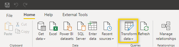
1. Open Power Query Editor
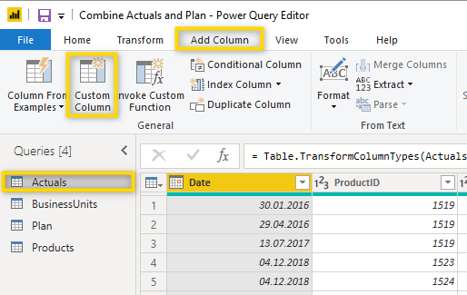
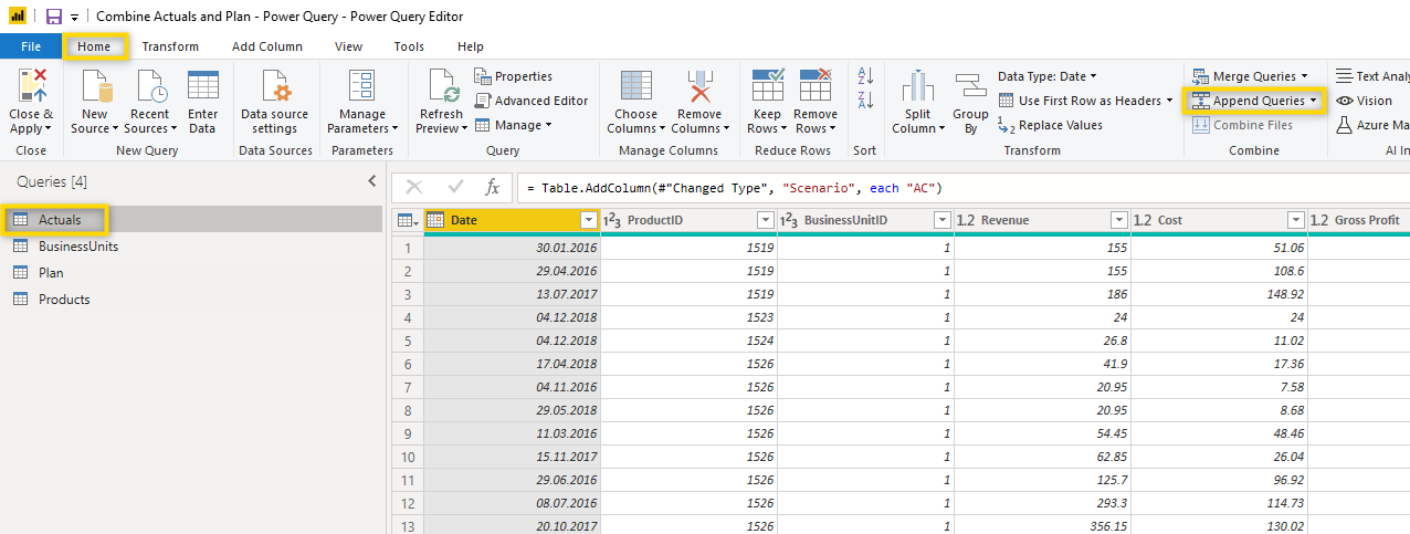
2. Add columns. In order to be able to distinguish Actual and Plan values after they have been combined into one table, we have to add a column to each of the existing tables which indicates the scenario. To add a column to the Actuals table, select the table and then select Add column > Custom column.
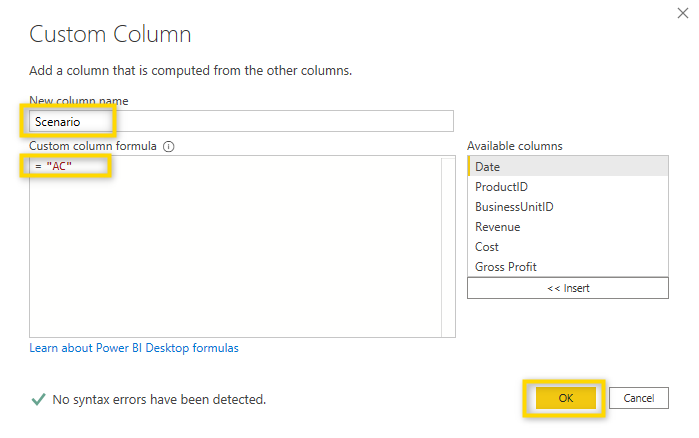
With the settings below, the new column is called Scenario and AC will be shown in every row.
Let’s do the same in the Plan table but this time add the value “PL”.
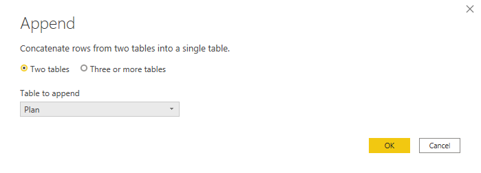
3. Combine tables into one. Let’s load the Plan data into the table with the Actuals. In order to do this, first select the Actuals table and then select Home > Append Queries.
Now you have to select from which table you want to load data.
⚠️ Before you append the queries, make sure that the column definition (name and data type) is identical for both tables.
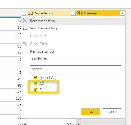
You now have all data (Actuals and Plan) within the table Actuals. In order to verify this, click the filter for the Scenario column and select Load more.
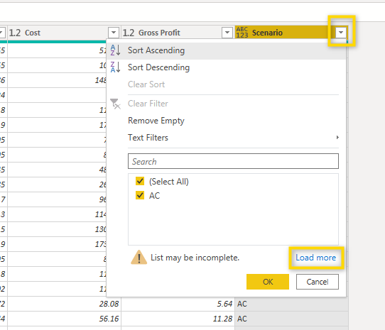
You will see that you have AC and PL values in the same table.
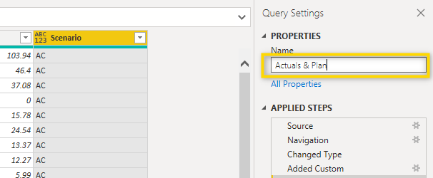
4. Now you need to rename the table to Actuals & Plan and make sure the Plan table isn’t loaded to the report anymore because it is no longer needed. You can rename the table in the properties on the right-hand side.
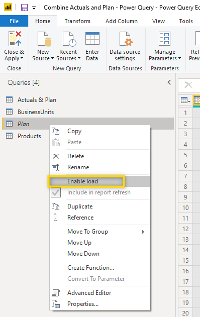
To disable the load of the Plan table, right-click it and uncheck Enable load.
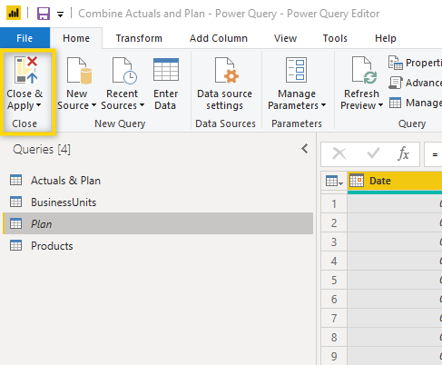
5. Load to Power BI. You are now ready to load all changes to Power BI. To do so, select Close & Apply.
When we look at the data model now, we can see that it is a proper star schema with three lookup tables and only one fact table.
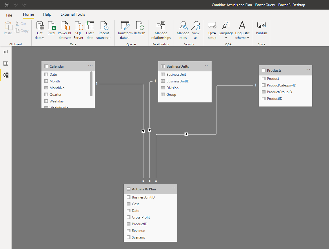
Having all transactions combined in one table will make the development of DAX measures and the overall setup of the report much easier.
Case 2: Combine Data with DAX TREATAS function
In this case, we assume that we have Plan data which is planned on a yearly level and only for Business Units but not for Products and Salesperson. This is what the data looks like:
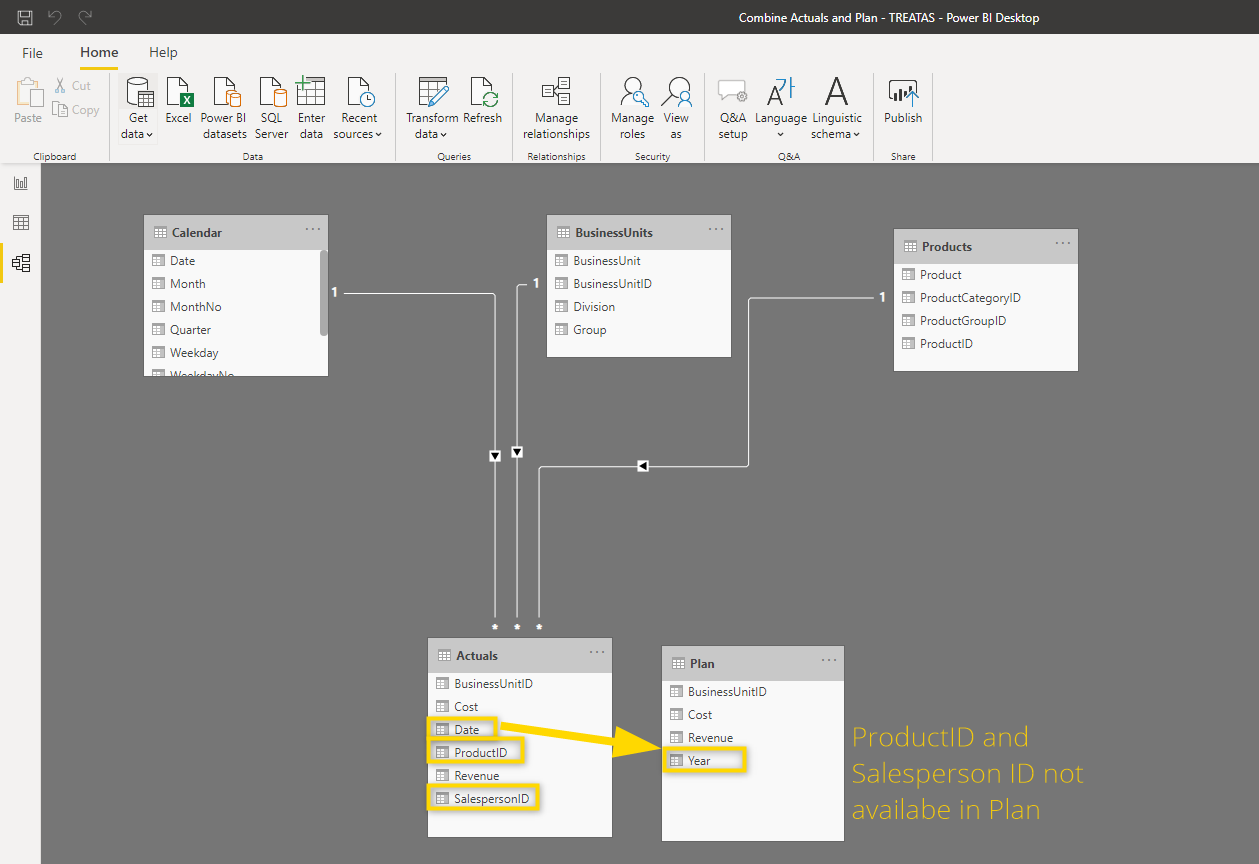
This means that we will not be able to compare Actuals with Plan for Products or Salesperson. Also, we will only be able to compare Actuals with Plan on a yearly level because this is the lowest common granular level.
When using the TREATAS function to combine Actuals and Plan, it’s important to note that the table with the plan data is not linked to any other table in the data model. The relationship will be done virtually using DAX.
1. Add the DAX function to be able to compare Actuals and Plan costs by year. The Measure for the yearly Budget looks like this:
Budget Costs (Yearly) =
CALCULATE(SUM(Plan[Cost]),
TREATAS( VALUES( 'Calendar'[Year]) , Plan[Year]))
Let’s break down this measure:
We use the CALCULATE function for most scenarios that are a bit more advanced. If you are not familiar with DAX measures, you can read the article about setting up basic measures.
Basically, the TREATAS function creates a virtual relationship between columns from different tables. The relationship we want to create is between the year column from the calendar table and the year column from the plan table. We are using the calendar table because that’s the table on which we base all our time filters and slicers in the report.
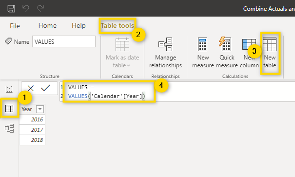
VALUES( 'Calendar'[Year])
The VALUES function creates a table that contains the unique values of the specified column. In order to better understand what it does, let’s see what the table looks like which is created with this function. You can do this in the Data view by selecting Table tools > New table. This formula creates a table that contains the years 2016, 2017, and 2018.
In (more or less) simple terms, what the above formula for the yearly budget does, is sum up all values in the cost column of the Plan table and makes sure it can be filtered by the year of the calendar table by creating a virtual relationship between the year of the calendar table and the year of the Plan table.
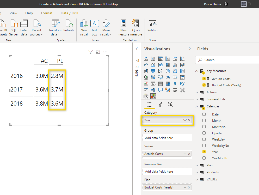
With this formula, we can compare Actuals and Budget per year.
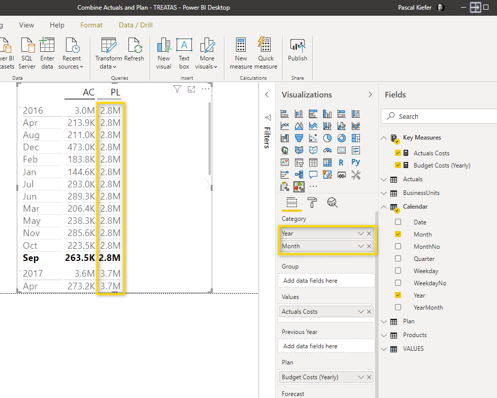
But let’s see what happens when we also add the months. The Plan values per month still show yearly values because there’s simply no monthly plan data available and we, therefore, couldn’t create a relationship. This is also, why we named the measure Budget Costs (Yearly) to make sure the end-users know that this is the lowest granularity.
2. Since we do have Plan data per Business unit, we should be able to also compare Actuals with Budget, right? Let’s see what happens when we pull in the Business Unit.
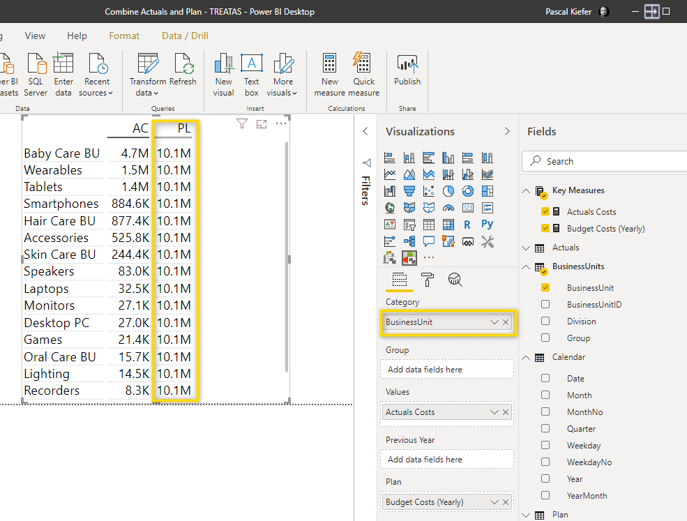
As you can see above, the Plan values per Business Unit are not correct. We should create the DAX measure that will make sure we can also show plan per Business Unit. The measure looks like this:
Budget Costs (Yearly & BU) =
	CALCULATE(SUM(Plan[Cost]),
	TREATAS( SUMMARIZE(Actuals, BusinessUnits[BusinessUnitID] , 'Calendar'[Year]), Plan[BusinessUnitID],
Plan[Year]))
The base calculation is still the sum of the values in the cost column of the plan table. Also, we still wrap everything in a CALCULATE statement. We also still use the TREATAS function, only this time we are creating two relationships. The first relationship is between the Business unit ID from the Business Unit table and the Business Unit ID from the plan table. The second relationship is between the year from the calendar table and the year from the plan table. The main difference is that the VALUES function has been replaced by SUMMARIZE.
This is what the table looks like which is created by the SUMMARIZE function:
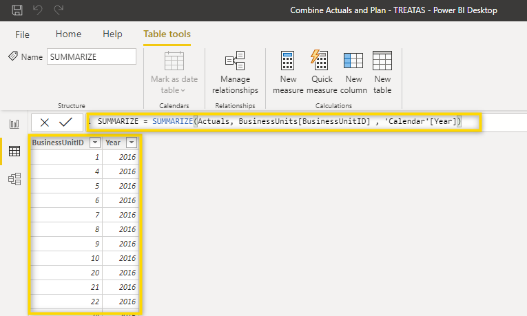
The table contains unique combinations of BusinessUnitID and Year which appear in the Actuals table. And this is exactly the table we use in the TREATAS statement.
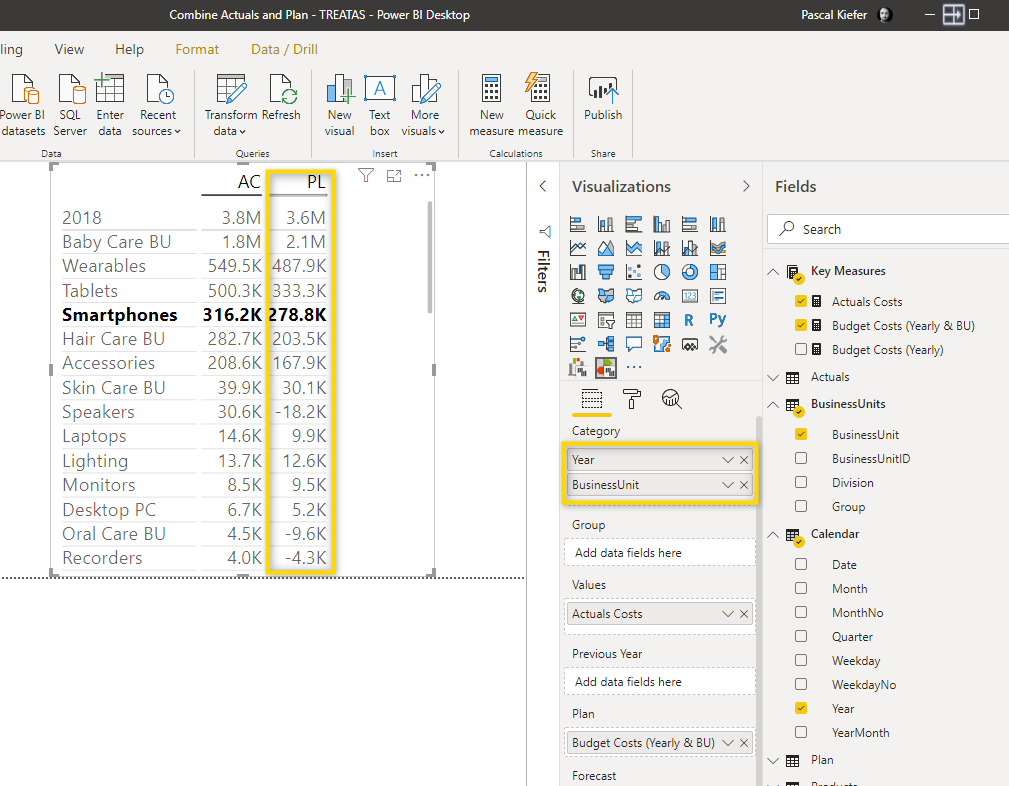
With this function, it is now possible to make the comparison per year and Business Unit.
We understand that there are many different reasons and scenarios why the granularity of Actual and Plan data is not identical and this article can not cover every possibility. But hopefully, this gives you an idea of how you could approach this problem and hopefully this will work for you.
Now that you have a fact table that contains all transactional data, it’s time to create some basic measures.