Imagine dynamic and interactive data exploration in Excel reports. Zebra BI enables you to connect many data tables, allowing you to filter and analyze data across various dimensions. With the ability to interactively drill down and study data from numerous angles, this feature improves data exploration. This way the report viewer may obtain a thorough understanding of their data, spot patterns, trends, and linkages, and make better-educated decisions with the help of cross-filtering.
Start from a simple Table
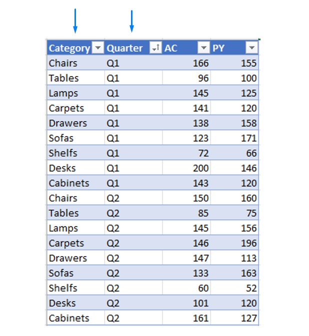
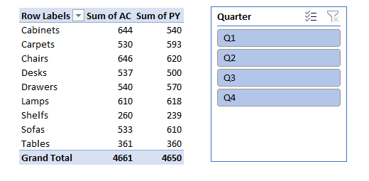
Here we have a Table in Excel containing two dimensions, one structural and one time-based. Our expected outcome is to visualize this data in two separate visual elements with the ability to filter data by clicking on a certain data point.
Creating Pivot tables
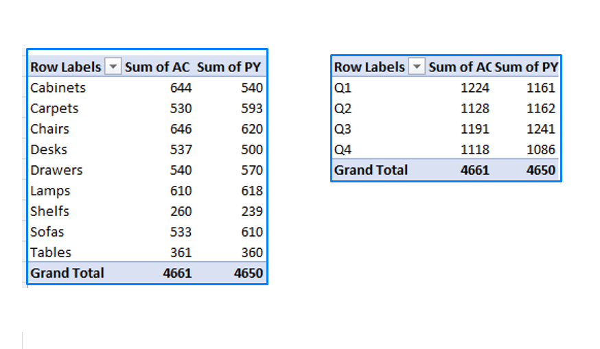
Next, we’ll create two separate pivot tables for each dimension. Click inside the table, go to the Insert tab, and under the Tables section click on PivotTables, where we select the first option – From Table/Range. A Pivot table can be placed on the existing worksheet or a new one, which is a default selection.

Creating Slicers
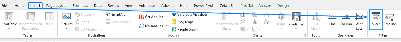
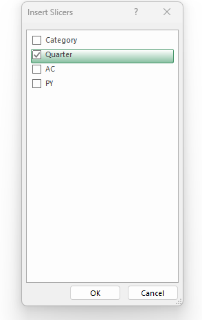
To create a slicer click inside any Pivot table and create a Slicer for each Pivot table, which is used to filter a certain Pivot table by the selected field. Once we insert a Zebra BI Add-ins from the Pivot table the slicer will connect to the Zebra BI Add-ins automatically. Go to the Insert tab and under the Filter section select a Slicer. When the pop-up window appears select a field by which you want to filter the specific Pivot table, click OK and the slicer will be created.
Any selection in the slicer is now reflected in the Pivot tables. Repeat this step for the other Pivot table.
Insert Zebra BI Add-ins
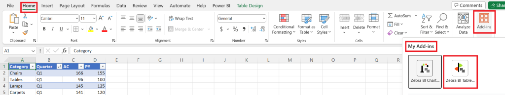
Once the slicers are done we can proceed to insertion of Zebra BI Add-ins. You can insert the free version by following the next steps:
- Click anywhere inside the table
- Move to the Home tab > Add-ins
- Select Zebra BI Tables for Office
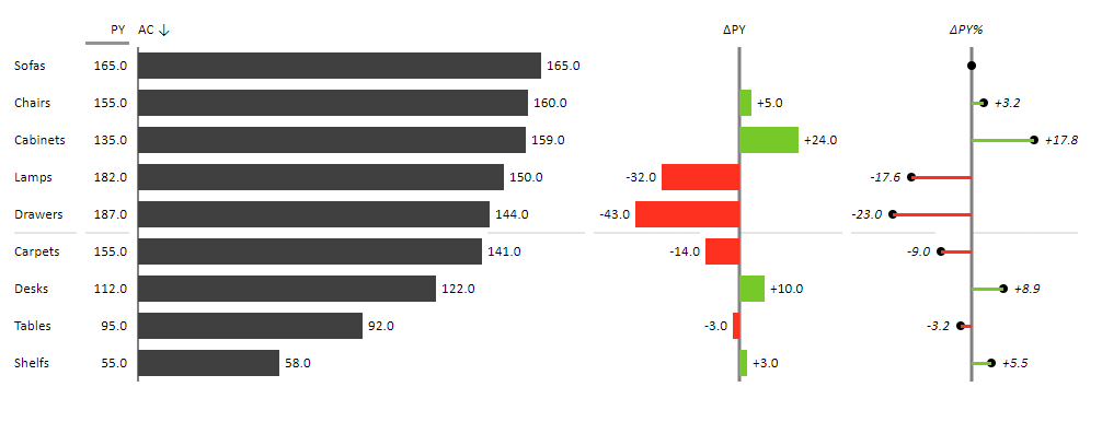
Your table will now look like this:
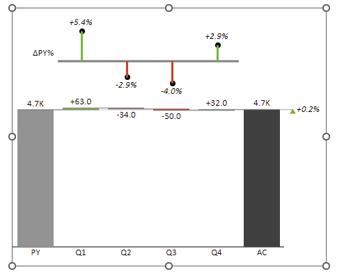
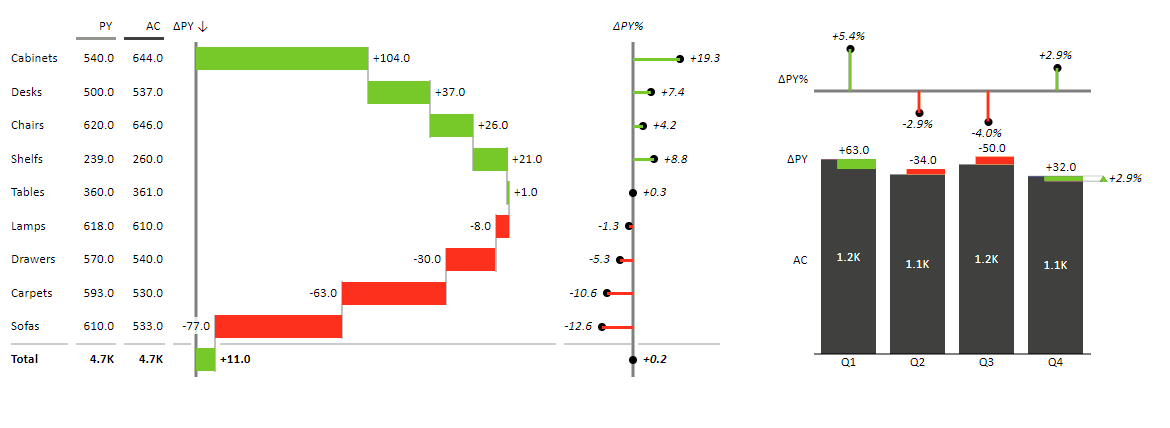
Repeat this step with the Quarter Pivot table but this time select Zebra BI Charts instead. The selection will render a waterfall chart by default, but there are many different chart types available on the Chart slider.
Start using the cross-filtering feature
As mentioned earlier, Zebra BI add-ins will detect the slicers and connections to Pivot tables automatically so any additional settings aren’t needed. Select any data point in the visual element to trigger the filtering.
In conclusion, Zebra BIs’ cross-filtering feature revolutionizes how data is evaluated and comprehended. This feature significantly enhances the flexibility, interactivity, and depth of data analysis in Excel, empowering you to extract valuable insights and drive impactful outcomes.