File used: Prepare file.xlsx
Our tools are easy to use. If you know how to insert the data into Excel, you will be more than capable of bringing amazing charts, graphs, and visualizations into Excel using Zebra BI for Office in Excel. We will use ranges, tables, and pivot tables as sources so you can start preparing and communicating your data effectively in minutes. Not hours, minutes.
You will learn how to prepare the data in 3 different formats:
- Ranges
- Excel Tables (recommended)
- Pivot tables
Let’s start with the basic one, ranges.
Ranges
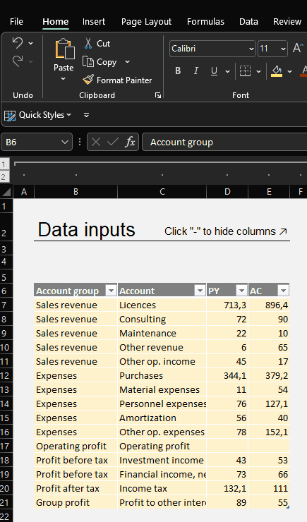
Template used: Sales monthly variances
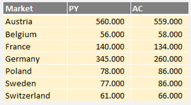
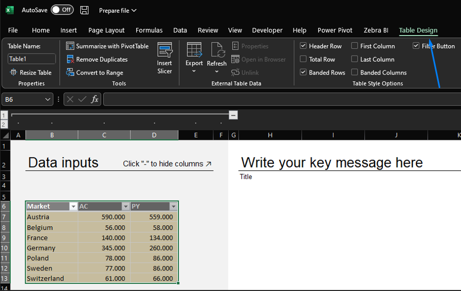
Excel ranges are ordinary data input on an Excel spreadsheet with a tabular format. Plain, and simple data as shown below:
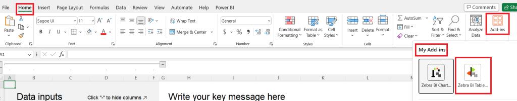
Let’s visualize it with the Zebra BI Tables for Office add-in in Excel. The requirement for visualizing this range of data is to have columns for Market (the category column), Actuals, and Previous Year (value columns). Let’s visualize it by following the steps below:
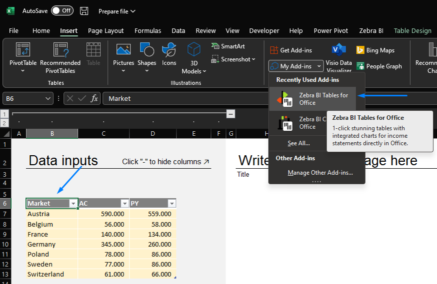
Check how to import Zebra BI for Office to Excel.
- Click anywhere inside the table
- Move to the Home tab > Add-ins
- Select Zebra BI Tables for Office
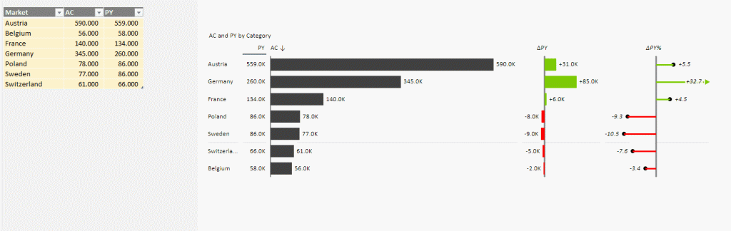
Let’s check the output:
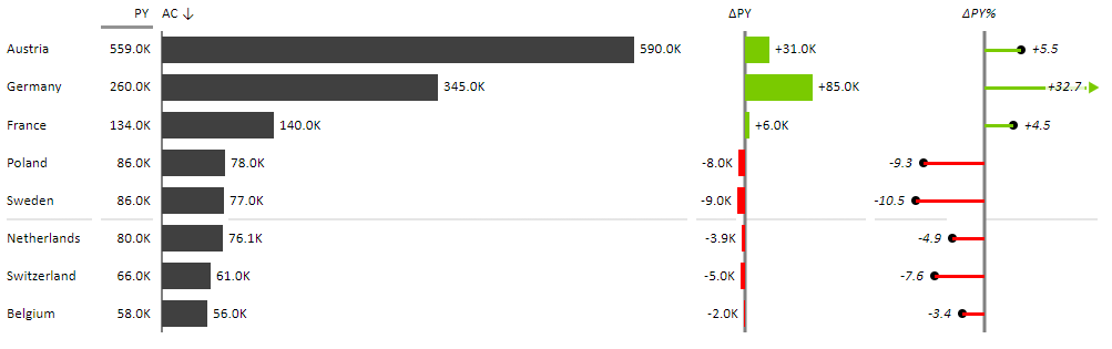
Let’s check how Zebra BI reads this data: correct column assignment article
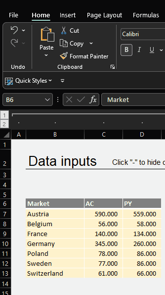
Updating the data is also supported. Let’s change Austria’s Actual (AC column) figure.
This feature is supported in all data sources, ranges, Excel tables, and pivot tables.
Excel ranges are powerful and easy to use. Updating the data in a range is limited, however. Entering new data rows is not supported. In that case, you should use Excel tables.
Excel tables (recommended)
The recommended source for Zebra BI add-ins in Excel is Excel tables. Using Excel tables is simple. Among other useful features, Excel tables will allow you to enter new data in the data source. Let’s create an Excel table first:
- Place your cursor within the data range
- Move to the Insert tab
- Select Table
CTRL + T is the shortcut for creating an Excel table. Note that the filters and a separate ribbon appear after you create an Excel table.
Great, you’ve created an official Excel table! Let’s create a visual from it:
- Place the cursor anywhere in the table
- Move to the Insert tab
- Add-Ins
- Insert the Zebra BI Tables for Office
Don’t forget to arrange your value columns to the correct placeholders.

Note that placing the cursor anywhere in the table vs the regular Excel range, we need to select the whole source by the cursor. Another advantage of using Excel tables is adding new rows. Let us add a new data row:
Note that the data is sorted ascending according to the AC column upon insertion. Double-click on the AC column to get the source data sorting.
Read more about sorting columns in Zebra BI Tables for Office.
In summary, Excel tables are recommended as the default data source because of their dynamic features, especially in adding new rows. To have more advanced visualizations, multi-level hierarchies, or small multiples, for example, we would need to use Excel pivot tables as the visual source.
Pivot tables
Pivot tables are one of the most powerful tools in Excel. One of the things it does well is summarizing and filtering your tabular data efficiently. Combined with Zebra BI for Excel you can create amazing hierarchical tables or small multiples charts. You can even combine it with your data model. Anything you can think of in pivot tables, even connect directly to Power BI datasets.
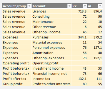
Let’s create a pivot table out of the following data, formatted as an Excel table:
Move to Insert -> PivotTable -> from Table/Range -> Existing worksheet -> Place it in cell T6
We get an empty pivot table in cell T6.
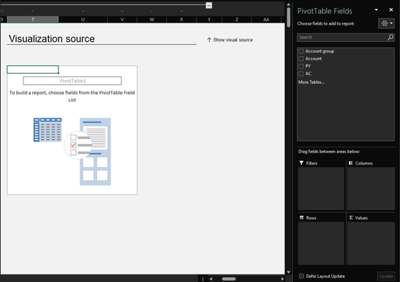
On the right-hand side pivot table fields pane is shown.
All columns from the source table are listed at the top. By dragging and dropping the columns to the areas below, we can create a pivot table.
Drag Account group and Account into Rows, PY and AC into Values:
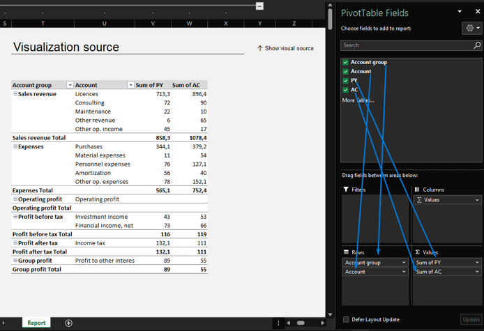
This is the ideal scenario for a multi-level hierarchy table (expand and collapse) visualization using the Zebra BI Tables visual. Place your cursor within the Pivot Table, and insert the Zebra BI Tables add-in.
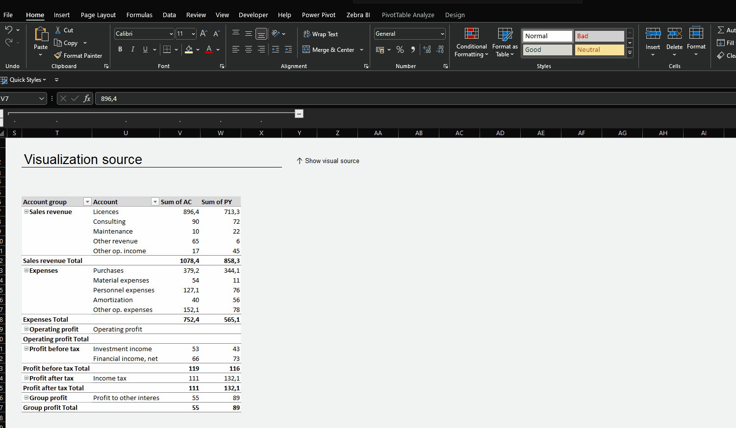
Click on the AC column header twice to apply the data source sorting.
An actionable income statement visual in seconds. This being a pivot table, adding new rows, and updating the data will be reflected after the PivotTable refresh.
The Zebra BI Tables custom formulas for Gross profit, Operating profit, and Net profit accounts are explained in the Zebra BI Tables for Office overview article. There you can learn more about waterfall charts in Zebra BI Tables for Office.
Here you can learn more about preparing an Income statement using the Zebra BI Tables add-in in Excel.
Changing the data source
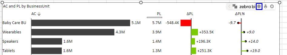
With Zebra BI visuals you have the ability to seamlessly switch between all 3 data source options (Range, Excel table, Pivot table). To do this simply hover with your mouse in the top right corner of the visual, expand the settings toolbar, and click on the cog icon:
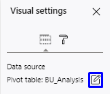
in the ‘Visual settings’ under ‘Data source’ click the edit icon:
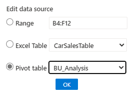
and select your desired visual data source:
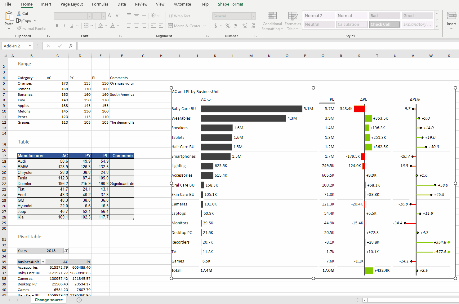
Here is a demonstration of the entire process:
Well done! You have learned how to prepare your dataset in ranges, tables, and pivot tables in Excel. Also, you now know how to update your data and reflect it in your visualizations. Keep in mind that the recommended data source for all Zebra BI add-ins in Excel and pivot tables is Excel tables.
You are now ready to turn your data into amazing reports in minutes.